Picoharp Guide

Principle

TCSPC measurements usually deals with time-resolved fluorescence spectroscopy. It can be used to capture the time decay profile of a signal from a single excitation-emission cycle. But instead of measuring only at one cycle, it extends the data collection over multiple cycles of excitation and emission. Using the ‘sparseness’ of the collected photons, we can reconstruct the fluorescence decay profile from the multitude of photon collection events.

In this picture, we can see that when an excitation pulse is applied, the time count begins, and the when the fluorescence photon arrives, the picoharp is able to measure the time difference, like a stopwatch.

The time difference is measured as follows: First there is a time window for a single experiment cycle. In the above picture, this time window is the time gap between two successive LASER pulses. Then, this time window is divided into small time bins, which is the resolution. Depending on the arrival time of the fluorescence photon, it collects the photon in a particular time bin, and in this way it accumulates a histogram, like the one shown below:

This measurement is reminiscent of a single-shot emission lifetime experiment. In our case, we shall be able to measure the single photon emission lifetime from the quantum dots, using the picoharp.

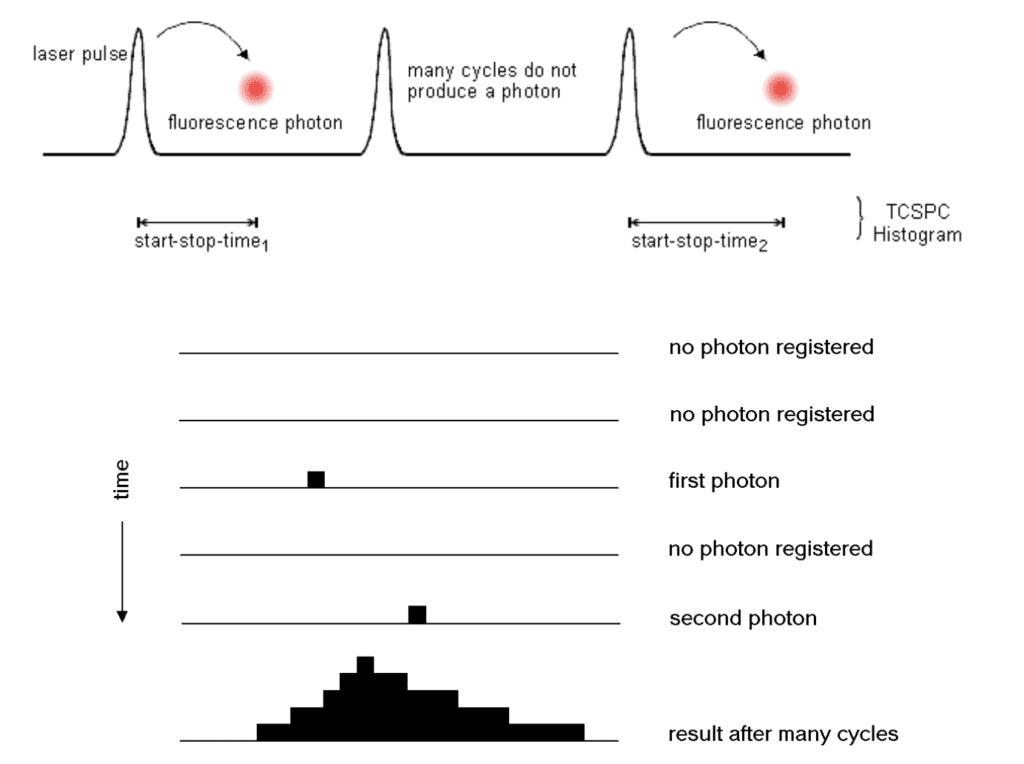
Another helpful illustration to understand the working of the picoharp would be following:

Usage

The picoharp has two channels: channel 0 and channel 1. Both of the channels are capable of measuring the count rates. It could the count rates of the photons, or it could also count the number of pulses, if a stream of pulses is applied to either of the channels. Basically, 1. If you apply a square pulse, with frequency f, it can count the frequency (which is basically the number of pulses, or counts per second), or, 2. It can actually count the number of photons, if the channel is connected with the single photon detector.

The picoharp has some maximum count rate, which is 10Mcps according to the document. The best timing resolution is 4 ps.

For acquiring the histogram, channel 0 is used as the synchronization signal (that defines the time window of one experiment) and channel 1 is used as the detector port, where the photons are counted. The sync signal can come from the LASER directly (some electrical signal that is generated from the LASER, synced with the LASER pulse), or, in our case, it can be generated using the AWG, and then this AWG signal can be used to synchronize the generation of the LASER.

Setting up Channel 0 (Sync Channel): The sync signal is usually a narrow negative pulse of -800 mV, terminating into 50 ohm. So, the sync signal we generate from the AWG must contain a negative polarity pulse. The negative pulse needs to be steep (0.5 to 10 ns wide). The optimum amplitude is -200 mV to -800 mV. There are some settings on the software of the sync signal (on the software, you can also set these using the MATLAB class, the use of which you will see below) called CFD, which is advised to be set at half of the sync amplitude initially. The zero cross voltage is advised to set at 10 mV initially. We can check with some square pulse signals if it shows the correct frequency (count rates) on the software/MATLAB. We can vary the discriminator level to have the correct value here. A last fine tuning of the discriminator and zero cross level as well as the sync offset can be
done when the detector input is up and running.

Setting up Channel 1: Channel 1 also accepts or reacts to negative polarity signal, but our single photon detector generates positive pulses. We have an inverter connected to the output of the detector, which takes care of this. We should initially set the CFD Discriminator Level to 30 mV and the CFD Zero Cross level to 10 mV.

As a matter of fact, channel 1 also accepts or reacts to negative polarity signal, but our single photon detector generates positive pulses. We have an inverter connected to the output of the detector, which takes care of this.

The picoharp takes negative pulses going from 0 to max -1 V. The optimum range of inputs is -100 to -500 mV. I don’t know how then it makes sense to say previously that the sync signal is usually a negative pulse of -800 mV…

Timing Requirements: You can have resolution (width of the time bin) starting from 4 ps upto 512 ps. The maximum count at one bin cannot exceed 65535. The time window of our experiment, as said earlier, will be dictated by the frequency or the period of the applied sync signal. I am not sure about, but I think the maximum time window (single experiment) permitted by the Picoharp is 33 us.

MATLAB Coding

Similar to very other instrument, we shall also use a MATLAB class to control various parameters of the Picoharp. It’s more handy to work with a code that can control many instruments, than to work with individual software.

The MATLAB class written for controlling the instrument is ClassPicoharp.m.

We also have some codes, that utilize the above class for various experiments that are usually repeatedly done. For example,

1. CheckCountStabilityDemo.m – a demo code that plots and saves the count rate of a specific channel as a function of time, at time intervals and until a final time defined by the user. Another application of this code could be, to change the center wavelength on the spectrometer, and see the change in the graph, that way we would be able to find the wavelength of the single photon emitter.
2. AcquireHistogramDemo.m – a demo code that plots and saves a histogram as a function of time, at time intervals and until a final time defined by the user. Saving the history of the experiment in such a way enables restoring useful data even if something in the experiment went wrong at a certain point.

Here are some familiarization on how to use the functions and the variables defined in the class:

1. X = ClassPicoharp.getInstance(): Creates an instance of the class, all the variables are functions are now contained inside X, which needs to be accessed using X.variable command.
2. X.connect(): Connection between the Picoharp instrument and MATLAB is established.
3. X.CloseConnection(): Closes the connection established between the Picoharp and the MATLAB.
4. X.SetResolution(Resolution): Defines the time resolution of our measurement.
5. In a similar way, we can set other parameters as well, like parameters ZeroCr0, ZeroDiscr0, ZeroDivider0, Offset0, ZeroOffset0, ZeroCr1, ZeroDiscr1, Block, Mode, Offset, TimeStop, CountStop.
6. a=X.GetResolution() – gets the resolution and returns into a.
7. a= X.ReadCounter(ChannelNumber) – reads the average count rate of a defined channel. Can be called multiple times for saving and plotting real-time information.
8. X. StartAcquisition() – starts acquiring histogram data from channel 1, given that a sync input was injected into channel 0. The default total acquisition time is the maximum permitted (360000 seconds). You can change this default value by launching X.SetTimestop(your final time) before you start acquiring, or by stopping the experiment on demand at any time using X.StopAcquisition()
9. X.StopAcquisition() – stops acquiring histogram data on demand at any time.
10. IsDone=X.CheckAquisitionDone() – checks if the acquisition is done.
11. [TimesVec,hist]=X.GetHistogram() – extracts the histogram data at the moment the command is launched. Can be called multiple times for saving and plotting real-time information. hist will get the histogram, and TimesVec will get the corresponding time vector in nanoseconds. The correct times are automatically calculated from the sampling resolution and frequency of the sync signal.