Imaging Polarimeter
1.0 Introduction
The goal of this instrumentation tutorial is to create and calibrate a Stokes imaging polarimeter. This requires a linear polarizer (polymer film will work) and a camera. Using a webcamera, cell phone, a point and shoot, or digital SLR camera, you will be able to collect image data. These data can be collected for any given scene using different polarizer orientations. You will then learn how to reduce the data and calculate calibrated (or approximately calibrated) Stokes parameters. I say “approximately” because most of these data will be collected using hand-held polarizers, and you can only position them so accurately!
2.0 Preliminary Setup
You will need to download two computer applications for this project. The first one is a small (free) application called “Iris”. It can be downloaded here: http://www.astrosurf.com/buil/us/iris/zip/iris.zip. The documentation is located here: http://www.astrosurf.com/buil/iris/nav_pane/CommandsFrame.html. This is a very powerful image processing software, mainly geared for (and created by) amateur astronomers – but it works great for other purposes too, and can be also used to process raw data from digital SLR cameras. You can also download and install Matlab or gain access to a computer that has it. Note that the required Matlab processing is fairly minimal, as much of it will be done in Iris (Note: for the purposes of the tutorial, we can use IRIS exclusively since Matlab is not free). Alternatively, Octave is like Matlab and is open-source. Much of the syntax is similar, so any discussion about Matlab can be applied to Octave as well.
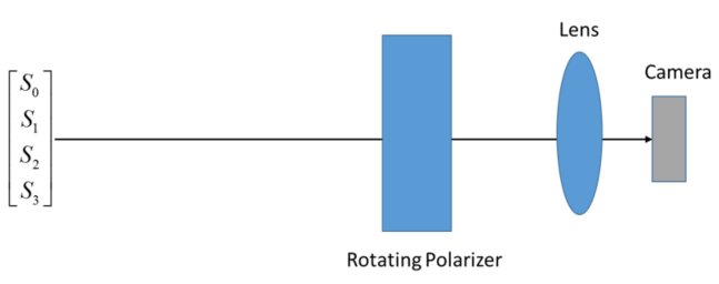
4.0 Configuration 1 – Linear Polarimeter
The first configuration that will be investigated is that of a simple linear polarimeter. In this case, it will consist of a rotating linear polarizer in front of a camera. The general configuration is shown below:
For this polarimeter configuration, it is recommended that you perform the following steps:
4.1 Collect Practice Data and Familiarize Yourself with Data Reduction Procedure
- Acquire 3 images of an indoor scene. This will allow you to collect some data so that you can practice the procedure. Ideally, hold the camera as still as possible to make image registration easier. One image should be taken through the rotating polarizer at 0 degrees, one image taken through the polarizer at approximately 45 degrees, and the final image should be acquired through the linear polarizer at 90 degrees. You can do this by holding the polarizer by hand in front of your chosen camera. Some tips are as follows:
- DIGITAL SLR: If you are using a digital SLR, put the camera on manual exposure (so fix the exposure speed AND focal ratio of the lens to something with acceptable dynamic range) and fix the white balance to daylight (actually, it does not matter what – just so long as it is fixed). For now, simply acquire data as JPG.
- SMARTPHONE: If you are using a smartphone, download a (preferably free) camera application that allows you to at least view the exposure speed, if not set it manually. The key is that you do not want the camera to automatically adjust the image brightness (gain) or to change the exposure speed during the course of your measurements. If you are having trouble with this, you may need to image the scene with some kind of diffuse target in it (like a piece of paper) that can be used to normalize the intensity of all the images. Ideally this target would also not produce a strong polarization signature. If you have an android phone, the app “Camera FV-5 Lite” works well: https://play.google.com/store/apps/details?id=com.flavionet.android.camera.lite. The free version restricts resolutions to 640×480 pixels, but this is sufficient for our purposes.
- POINT AND SHOOT: For point and shoot cameras, the control over the exposure, focal ratio, white balance, etc. is highly varied. Try to place the camera in “as manual” a mode as possible. For instance, many cameras have aperture priority or shutter priority modes – these can be better than full automatic. Additionally, most have a way to manually set the white balance, so you will want to enable this option if available. Finally, some cameras have “picture modes” (somewhat obscure modes on the cameras, like “night shot”, etc.) that can enable manual features. Please see me if you are having difficulty maintaining the exposure and/or focal ratio from shot to shot.
- WEBCAM: For most web camera applications, you have control over the exposure, gain, white balance, etc. So you should be able to control the exposure. But again this can vary from camera-to-camera.
Of these options, the digital SLR is the suprior, followed by the webcam and/or point-and-shoot, with the smartphone coming in last. For best results, as much control over the exposure, white balance, exposure bracket, etc. is needed.
Below is an example of 3 images that I took using the FV-5 Lite camera application using my android cellphone camera. This is a 3 exposure series of my office desk (super exciting!).
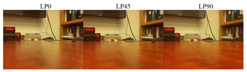
Note the reflection of the wall on the desk – it is decreasing its intensity as the linear polarizer is rotated from 0 degrees (the reflected s polarized light from the desk transmits) to 90 degrees (the reflected s polarized light from the desk gets blocked). The 45 degree position is somewhere in between.
- Transfer the files to your computer into a dedicated directory (e.g., C:\tempimages\linearfiles\). Within this directory, create a temporary folder (e.g., C:\tempimages\lienarfiles\tmp\). This folder is where Iris will store its temporary and intermediate image files.
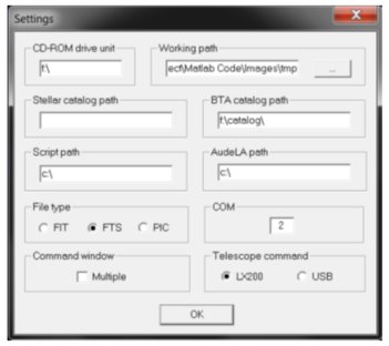
- Open Iris. Within Iris, select “File -> Settings” and select “Working Path”. Copy and paste the path to the temporary directory to this location (e.g., C:\tempimages\lienarfiles\tmp\). Also select FTS under “File Type”. FTS or FITS files are used commonly by NASA and can be loaded easily into Matlab. Click OK to close the dialog box.
- Now open the first image that you saved (say, your LP0 image). This is straightforward and can be done from the menu bar – when opening, be sure to select “Files of type:” and select “graphics”.
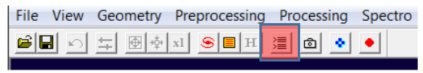
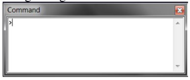
- Open the command line. This is the small text looking button on the menu bar:
This will open the following dialog:
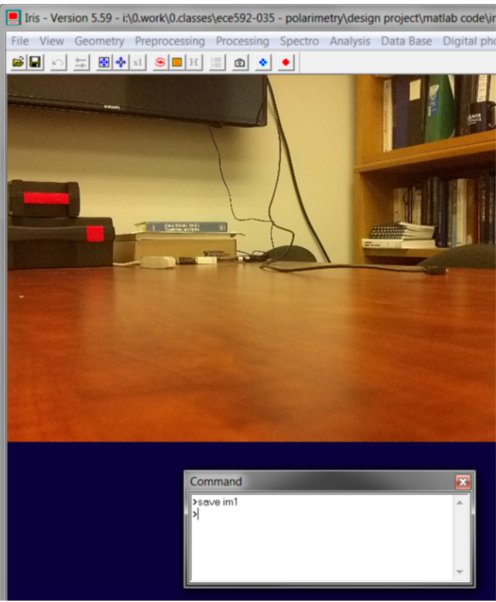
- Now you will save the images as FTS files. These will be saved in the tmp folder for future use. Simply type “save im1” to save the first image as an FTS.
- Repeat steps 4 and 6 on the other two images (LP45 and LP90). Save LP45 as im2 and LP90 as im3.
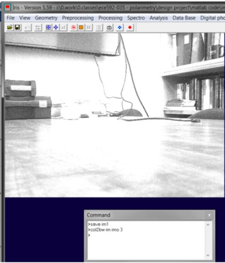
- Now you will convert the images to grayscale by summing the RGB values for each pixel (this is the inherent way that Iris creates the conversion). We will then divide the image by 3 so that we retain the previous dynamic range (0 to 255 in most cases). To convert to grayscale, first open im1 by typing
load im1
in the command line. Then, convert the image to grayscale by typing:
col2bw [INPUT] [OUTPUT] [NUMBER]
In this case, input is the [input] is the input image’s PREFIX (in this case, im), the [output] is the output image’s PREFIX (something other than im, say, imo), and number is the number of images that you want to convert within the series (in this case, 3). So we would type:
col2bw im imo 3
Iris will perform the batch conversion, yielding the over saturated grayscale image below. Note that this is only over saturated because in IRIS the default maximum value is 255. You can select “Auto” on the “threshold” toolbar and it will rescale the image’s dynamic range (remember, the RGB values were ADDED together, so the maximum value in the image can now be 255*3).
- Now divide the images by 3. First, the images must be opened. Simply type
load imo1
To load the first image into the workspace. Then click on “Processing” and select “Divide” and under “Value” enter 3. This will produce an image that is bounded by 0 to 255, as was the case in the original image. Once this is completed, type in the command line:
save imo1
Which will simply replace the active image with the previous image on the hard drive.
- Perform the previous step for images imo2 and imo3 such that all 3 images have been divided by 3.
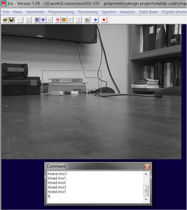
- Finally, you need to take your 3 images and perform spatial image registration. This is best done to better than 1/10th of a pixel (which is actually quite hard to do). Iris can do a pretty good job of registering images, which is the primary reason why we are using it. In the command line, type
open imo1
to load the first image into the workspace. Now select an area in the middle of your image (it can also be slightly decentered). The key is that it must have spatial information within it – so areas with edges, etc. are good in my image, but the area around the desk would be a poor choice. An example is shown below:
Now select “Processing” and choose “Planetary Registration (1)”. This will open the following dialog:
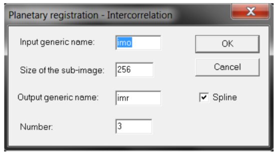
In this box, type “Input Generic name” as imo (again, this is the INPUT prefix), leave the sub-image size as 256 pixels, and under “Output generic name” type imr. Finally, for number, select 3 since we have 3 images (e.g., imo1, imo2, and imo3). If we had 10 images, we would simply type 10 here – so this is just dependent on how many images you have in your current sequence. Clicking OK will register the images and save the spatially registered output images in imr1, imr2, and imr3.
- Congrats! You have navigated your way through IRIS. The program is very powerful for processing images. It also has some good noise filtering functionality and it can also handle RAW images from digital SLR cameras very very well!
- MATLAB for Stokes parameter calculation (Optional – Note you can also do this in Octave): Now you can transition into using Matlab. You could technically continue to use IRIS for the rest of this, but it may be more cumbersome than it needs to be. In any case, the Matlab script is straightforward and mainly requires that you input the correct measurement matrix (W). The Matlab code that I have prepared is provided in Appendix A. The code is generally setup as follows:
- Load the 3 images into an array “Samples” that is Nx x Ny x Ns, where Nx and Ny are the number of pixels in x and y for your particular camera and Ns is the number of images (in this case, 3).
- Create the W matrix. In this case, a function “lpr” is used, which is a custom function of mine. This simply takes three inputs, the orientation of the diattenuator’s transmission axis in degrees, the transmission of the x axis, and the transmission of the y axis, and provides you with a Mueller matrix of the diattenuator.
- Apply the W matrix inversion technique to EACH PIXEL of the sample data.
- Once completed, the Stokes vector is stored in a matrix S which is Nx x Ny x 4 with the implication that the S3 component is always 0 (this is a linear polarimeter).
- The DOLP is then calculated, along with the normalized Stokes parameters. These can then be displayed with Matlab.
- IRIS for Stokes parameter calculation: If you really want to use IRIS to calculate the Stokes parameter images, you can. However, you will need to determine the pseudoinverse of the W matrix before you do so. In this case, W is:
W =
0.5050 0.4950 0 0
0.5050 0.0000 0.4950 0
0.5050 -0.4950 0.0000 0
And the pseudoinverse PW is:
PW =
0.9901 0.0000 0.9901
1.0101 0.0000 -1.0101
-1.0101 2.0202 -1.0101
0 0 0
From PW, we can apply the coefficients in IRIS using the multiply command. The first row of PW calculates S0, the second row calculates S1, third row S2, and fourth row S3. Each coefficient multiples imr1, imr2, and imr3. Thus, to calculate S0, we can perform the following in the command window below:
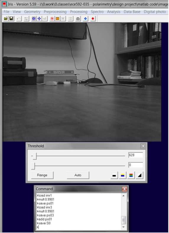
In this case, im1 is loaded, multiplied by 0.9901, saved as pr01. Im3 is then loaded, multiplied by 0.9901, saved as pr03. Then pr01 is loaded and added to pr03 and saved as S0.
Similarly, S1 can be calculated:
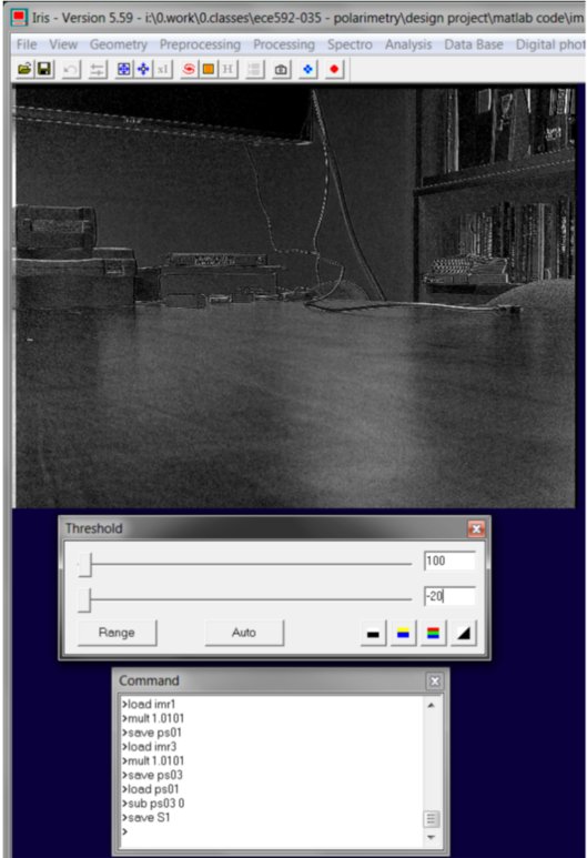
Note that S1 is very dominant on the horizontal desk. This is because most of this light is polarized horizontally (s polarized) in this case.
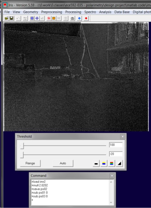
Finally we can process S2: (note ps01 and ps03 were calculated in the previous step for S1).
You can also do division to calculate the normalized Stokes parameters, but ultimately this will get a bit challenging to do in Iris as opposed to Matlab primarily due to divide by 0 or large pixel values (infinity).
4.2 Collect Indoor Validation Data
Perform the same procedure as in Section 4.1 on a “validation scene”. In this case, the simplest validation is to check if your degree of linear polarization is greater than one. The easiest scene to see with a DOLP of 1 is your laptop, TV, or computer screen. This contains a linear polarizer which is usually oriented (approximately) at 45 degrees. For these images, be careful to make sure that the laptop screen is relatively far away so that you can perform image registration on some other part of the scene (say, something behind the laptop screen). If you try to use the laptop screen itself (or the information on it) to perform the image registration step, it won’t work on some frames because the laptop screen may be completely dark! Process the data and verify that the DOLP is approximately equal to 1.
4.3 Collect Outdoor Data
Now you can go outside and collect some images. Interesting objects include cars and parking lots. Pavement also has an interesting polarization signature, as well as water. Be careful about trees, though. One issue with a temporally scanned polarimeter such as this are trees and wind. This can cause issues with image registration (if you try to use a tree as your registration target) or it can create false polarization signatures (the trees will look more polarized than they should be!).
4.4 Color Fusion
While we won’t cover it here yet, these results can be depicted in a Red Green and Blue colorspace. In a colorfused image, the grayscale intensity (S0) image is falsely colorized using the polarization information. Specifically, the degree of linear polarization (DOLP = sqrt(S1^2+S2^2)/S0) is used to establish the saturation, or amount of color, for a given pixel. Meanwhile, the orientation of the linear polarization state is used to establish the hue, or color, of a given pixel. A view of an image from the Hunt Library at NCSU, taken by Brett Pantalone, illustrates this effect.
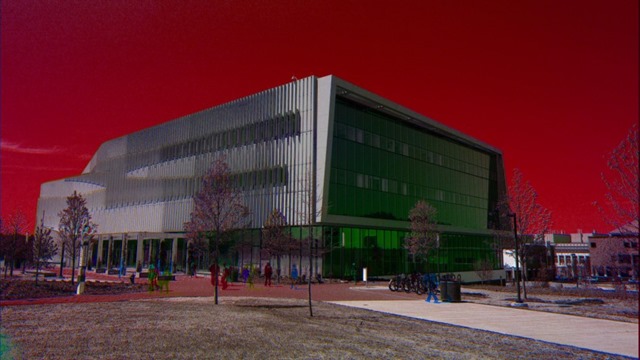
Note that the sky in the background is polarized, as indicated by the presence of highly saturated color. This polarization is due to Rayleigh scattering in the atmopshere, and is what many insects use for navigation. Meanwhile, the window surfaces on the building (smooth dielectric surfaces) are also highly polarized, but have a different color (green). This indicates that it has a similar polarization strength (similar degree of linear polarization) as the sky; however, it is polarized at a different angle. In this case, green is roughly vertically polarized while red is roughly polarized at 135 degrees. Conversely, rough surfaces in the scene, such as the pavement and grass, are generally unpolarized or weakly polarized as indicated by the relative lack of color. Finally, you can also see colorful “shadows” of people. This is actually caused by the temporally scanned nature of the polarimeter. Since it takes time to rotate the polarizer into new orientations, movement in the scene (as is generated by people walking past the camera) shows up as a false polarization signature!
5.0 Appendix A – Matlab / Octave Reduction Matrix Code
clear all
close all
%load images
tmp = fitsread(‘I:\0.Work\0.Classes\ECE592-035 – Polarimetry\Design Project\Matlab Code\Images\tmp\s2.fts’);
Samples(:,:,1) = tmp;
tmp = fitsread(‘I:\0.Work\0.Classes\ECE592-035 – Polarimetry\Design Project\Matlab Code\Images\tmp\s1.fts’);
Samples(:,:,2) = tmp;
tmp = fitsread(‘I:\0.Work\0.Classes\ECE592-035 – Polarimetry\Design Project\Matlab Code\Images\tmp\s3.fts’);
Samples(:,:,3) = tmp;
Nx = length(Samples(:,1,1));
Ny = length(Samples(1,:,1));
Ns = length(Samples(1,1,:));
%%
%now calculate the Stokes parameters assuming that the linear polarizer has
%an extinction ratio of 100 or so.
M1 = lpr(0,1,0.01);
M2 = lpr(45,1,0.01);
M3 = lpr(90,1,0.01);
W(1,:) = M1(1,:);
W(2,:) = M2(1,:);
W(3,:) = M3(1,:);
PW = pinv(W);
%reconstruct the Stokes parameters pixel by pixel, using the registered
%images
Pout = zeros(Nx,Ny,Ns);
Pout(:,:,1) = Samples(:,:,1); %this was the master image from before
for n=1:Nx
n
for m=1:Ny
%create power vector
P = squeeze(Samples(n,m,:));
S(n,m,:) = PW*P;
end
end
%%
S0 = flipud(squeeze(S(:,:,1)));
S1 = flipud(squeeze(S(:,:,2)));
S2 = flipud(squeeze(S(:,:,3)));
S1norm = S1./S0;
S2norm = S2./S0;
DOLP = sqrt(S1norm.^2+S2norm.^2);
figure(1)
imagesc(S1norm)
colormap(gray(256))
caxis([-1 1])
figure(2)
imagesc(S2norm)
colormap(gray(256))
caxis([-1 1])
figure(3)
imagesc(DOLP)
colormap(gray(256))
caxis([0 1])
[1] Care must be taken when using this polarimeter configuration, though, because the polarization state that is incident on the camera is always changing – this can result in additional measurement error!
[2] For truly accurate data with a digital SLR, you can also acquire images in RAW mode – but processing steps will differ significantly if you do this. So please for now, use JPG.
This material is based upon work supported by the National Science Foundation under Grant Number (NSF Grant Number 1407885). Any opinions, findings, and conclusions or recommendations expressed in this material are those of the author(s) and do not necessarily reflect the views of the National Science Foundation.